Linear regression model is one of the most widely used statistical/machine learning model, because of its simplicity for model interpretation. This post will discuss about how to interpret a linear regression model after transformations. Let’s consider the simple linear regression model first:
where the coefficient gives us directly the change in y for a one-unit change in x. No additional interpretation is required beyond the estimation of .
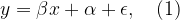
However, in certain scenarios, transformation is necessary to make the model meaningful. For example, one important assumption under the linear regression model is the normality of the error term in (1). If the observations of the response y is skewed (e.g., house price and travel expenses, etc.), then a log transformation is often applied to make it closer to normal. Another reason to apply a log transformation could be the inherent relationship between x and y is just not linear. The figure below shows how the log transformation is used to convert a highly skewed distribution to a close to normal distribution.
Left: histogram of y which is highly skewed; right: histogram of log(y) which is close to normal
When the response y is log-transformed, (1) becomes the so called log-linear model:
Note that the log(-) above means the natural log. In this case, what does the value of mean? Let’s consider two observations and :
Every unit change in x would result in change in the response y. In addition, when the estimated coefficient is small (close to zero), the percent change in y is approximately . For example, if , then 1-unit change in x would result in 5% change in y.
In conclusion, coefficient in the log-linear model represents a relative change in the response y for every unit change in x.


![log(y_2)-log(y_1)=\beta (x_1+1) - \beta x_1 + \alpha - \alpha \\[8pt] \Rightarrow log(\frac{y_2}{y_1}) = \beta \\[8pt] \Rightarrow \frac{y_2}{y_1} = e^{\beta} \\[8pt] \Rightarrow \frac{y_2-y_1}{y_1}=e^{\beta}-1 \approx \beta, \quad when \quad \beta \rightarrow 0. \quad (3)](https://s0.wp.com/latex.php?latex=log%28y_2%29-log%28y_1%29%3D%5Cbeta+%28x_1%2B1%29+-+%5Cbeta+x_1+%2B+%5Calpha+-+%5Calpha+%5C%5C%5B8pt%5D+%5CRightarrow+log%28%5Cfrac%7By_2%7D%7By_1%7D%29+%3D+%5Cbeta+%5C%5C%5B8pt%5D+%5CRightarrow+%5Cfrac%7By_2%7D%7By_1%7D+%3D+e%5E%7B%5Cbeta%7D+%5C%5C%5B8pt%5D+%5CRightarrow+%5Cfrac%7By_2-y_1%7D%7By_1%7D%3De%5E%7B%5Cbeta%7D-1+%5Capprox+%5Cbeta%2C++%5Cquad+when+%5Cquad+%5Cbeta+%5Crightarrow+0.++%5Cquad+%283%29&bg=ffffff&fg=000000&s=1&c=20201002)


